
Bode plots are diagrams used to analyze transfer functions (the ratio between an output function and an input function). The diagrams plot the magnitude and phase of the expressed function versus frequency. See Bode plot for more information.
This instrument has two main areas, the control area and the plot area.
The control area contains items to adjust the generated signal and to select visualization options.
When the instrument is started, the Scope and WaveGen Channel 1 are stopped and their status shows Busy. The Network Analyzer instrument takes control over the selected channels while running.
The control area lets you adjust the settings for the Bode analysis.
With "Use Channel 1 as Reference" option checked (default), oscilloscope channel 1 should be connected to the filter input and will be used as a reference to calculate the filter magnitude and the phase measured with the other scope channels. Without this option gains of each channel will be calculated relative to the set AWG amplitude and no phase calculated.
The analysis is performed from start to stop frequency in the specified number of steps. For each step the WaveGen is set to a constant frequency and the Oscilloscope performs an acquisition. Using the FFT result from the index corresponding to the current frequency step, the magnitude and phase value is calculated. The magnitude of Channel 1 (Filter input) is calculated relative to AWG Amplitude and other channels relative to Channel 1. The magnitude is expressed in decibels with the 20 * Log10 (gain) formula, where 1x gain equals 0dB and 2x gain equals ~6dB. The phase is plotted with the maximum value as the one specified for the Phase Top value.
The context menu is shown for the active view. It contains options available for the view.
The Bode plot shows the magnitude and phase.
Channel 1 magnitude is relative to the selected gain under Scope channels. The other channels magnitude and phase values are relative to channel 1.
The drop-down button in the top-right corner (or mouse right-click) shows the following options: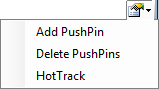
The HotTrack lets you take measurements by moving the mouse cursor. This shows a vertical cursor and the values at intersections with waveforms. The corresponding position is marked with a cross on Nichols and Nyquist plots.
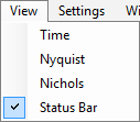
The time plot shows the oscilloscope acquisition of the last frequency step. This view is used to help adjusting the offset and gain of the oscilloscope input channels.
The Nichols plot is the magnitude and phase plotted in the Cartesian coordinate system.
The Nichols plot is the magnitude and phase plotted in the polar coordinate system. The scale is based on Max-Gain or Scope Channel Gain settings.
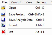
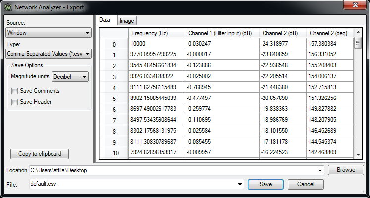
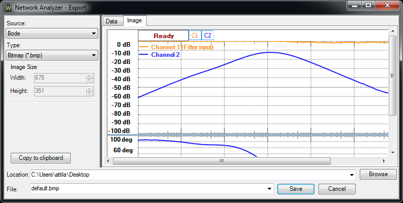
The Export dialog lets you save the data or screenshot.
You can export acquisition data by clicking File/Export in the plot window.
The data can be saved in CSV (Comma Separated Values) or TXT (Tab Delimited Values) formats. By checking the save options, the following information will be also saved:
In order to import the CSV file in Mathworks-MatLab, with csvread function uncheck Comments and Header, for DesignSoft-TINA application check both.
The plot window image can be saved in BMP (Bitmap), PNG (Portable Network Graphics), GIF (Graphics Interchange Format), TIFF (Tagged Image File Format), JPEG (Joint Photographic Experts Group) or EPS (Encapsulated PostScript) formats.
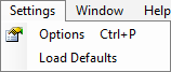
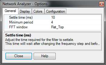
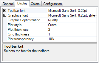
From the Settings menu, choose Options.
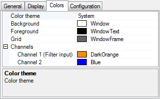
The Colors tab lets you select the color options for: background, text, axis, and channels.
Changing the Color Theme loads a default set of colors.
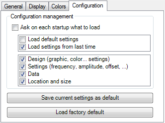
Ask on each startup what to load: lets you select whether the default or last configuration is loaded at start-up, as well as which items to configure.
Save current settings as default: saves the settings you have selected as default.
Load factory default: restores the default settings.